One of the most important concepts when designing and analyzing algorithms is time complexity. It measures the amount of time an algorithm takes to run relative to the size of its input. Time complexity helps us predict how an algorithm will scale and perform as the input grows, which is crucial when working with large datasets.
In this article, we’ll explore time complexity, how it’s measured, and the different notations used to express it.
Table of Contents
What is Time Complexity?
Time complexity represents the computational cost in terms of time as a function of the input size, usually denoted as n. It helps answer the question: How much longer will this algorithm take if the input size doubles?
The efficiency of an algorithm is determined by how its time consumption grows as the input size increases. An algorithm with poor time complexity might work well with small inputs but can become prohibitively slow as input size grows.
Big-O Notation: The Gold Standard
The most common way to describe time complexity is with Big-O notation, which gives an upper bound on the time an algorithm will take in the worst case.
Big-O notation ignores constants and lower-order terms, focusing only on the term that grows the fastest as the input size increases. For example, an algorithm that takes 5n² + 3n + 2 steps is said to have O(n²) time complexity because the n² term dominates for large n.

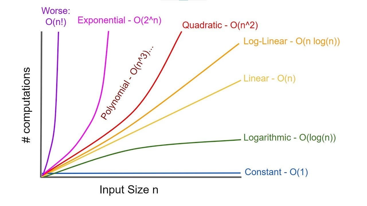
Common Time Complexities:
O(1) – Constant Time:
- Example: Accessing an element in an array by its index.
- The runtime is constant and does not change with the size of the input.
O(log n) – Logarithmic Time:
- Example: Binary search.
- The runtime increases logarithmically as the input size increases, making it efficient for large datasets.
O(n) – Linear Time:
- Example: Iterating over all elements in an array.
- The runtime increases linearly with the input size, i.e., if the input doubles, the time taken doubles.
O(n log n) – Linearithmic Time:
- Example: Merge sort, quicksort (average case).
- The runtime increases at a rate proportional to n * log(n).
O(n²) – Quadratic Time:
- Example: Bubble sort, selection sort.
- The runtime increases quadratically with the input size. It is slow for large inputs, and often inefficient for datasets beyond a few thousand elements.
O(2ⁿ) – Exponential Time:
- Example: Recursive algorithms that solve the Tower of Hanoi.
- The runtime doubles with each additional element in the input. Not suitable for larger inputs
Understanding Time Complexity with Examples
| Complexity | Name | Growth Rate Example | 1 Item | 10 Items | 100 Items | 1000 Items | 10,000 Items |
|---|---|---|---|---|---|---|---|
| O(1) | Constant | Stays the same | 1s | 1s | 1s | 1s | 1s |
| O(log n) | Logarithmic | Grows slowly | 1s | 2s | 3s | 4s | 5s |
| O(n) | Linear | Grows proportionally | 1s | 10s | 100s | 1000s | 10,000s |
| O(n²) | Quadratic | Grows as square | 1s | 100s | 10,000s | 1,000,000s | 100,000,000s |
| O(2ⁿ) | Exponential | Grows exponentially | 2s | 1024s | 1.27 × 10³⁰ s | 1.07 × 10³⁰¹ s | Practically infinite |
Key Observations:
- O(1) is the best case (fastest, independent of input size).
- O(log n) is very efficient, often seen in searching algorithms.
- O(n) is manageable but can get slow for large inputs.
- O(n²) is inefficient for large inputs, common in brute-force approaches.
- O(2ⁿ) is impractical for anything beyond small inputs.

How to Calculate Time Complexity?
To calculate time complexity, break down the algorithm into basic operations and count how many times they are executed as a function of input size n. Let’s take a few examples:
Example 1: Iterating Over an Array
def print_elements(arr):
    for element in arr:
print(element)- The
forloop runs n times, where n is the number of elements inarr. - Each iteration performs a constant-time operation (printing).
- Thus, the time complexity is O(n) (linear time).
Example 2: Nested Loops
def print_pairs(arr):
    for i in range(len(arr)):
        for j in range(len(arr)):
print(arr[i], arr[j])- The outer loop runs n times.
- The inner loop also runs n times for each iteration of the outer loop.
- This results in a total of n × n = n² iterations, giving the time complexity O(n²) (quadratic time).
Example 3: Binary Search
def binary_search(arr, target):
    low, high = 0, len(arr) - 1
    while low <= high:
        mid = (low + high) // 2
        if arr[mid] == target:
            return mid
        elif arr[mid] < target:
            low = mid + 1
        else:
            high = mid - 1
return -1- Each step of the binary search cuts the input size in half.
- The time complexity is logarithmic, O(log n).
Example 4 Identify the Dominant Term
def complex_algorithm(arr):
    n = len(arr)
    # O(n) operation
    for i in range(n):
        print(i)
    # O(n^2) operation
    for i in range(n):
        for j in range(n):
print(i, j)- When combining different parts of the algorithm, focus on the term that grows the fastest as
nincreases (this is the dominant term). - The time complexity of this algorithm is O(n + n²), but the quadratic term dominates as
ngrows, so the overall complexity is O(n²).
The time complexity of common algorithms
Sorting algorithms
| Algorithm | Best Case | Average Case | Worst Case | Notes |
|---|---|---|---|---|
| Bubble Sort | O(n) | O(n²) | O(n²) | Simple but inefficient; avoids swaps if already sorted (best case) |
| Selection Sort | O(n²) | O(n²) | O(n²) | Always performs the same number of comparisons |
| Insertion Sort | O(n) | O(n²) | O(n²) | Efficient for small or partially sorted data |
| Merge Sort | O(n log n) | O(n log n) | O(n log n) | Divides the array and merges; stable sort |
| Quick Sort | O(n log n) | O(n log n) | O(n²) | Highly efficient, but worst case can be quadratic; randomization improves performance |
| Heap Sort | O(n log n) | O(n log n) | O(n log n) | In-place and uses a heap data structure |
| Counting Sort | O(n + k) | O(n + k) | O(n + k) | Only works with small integer ranges (k is the range of input) |
| Radix Sort | O(nk) | O(nk) | O(nk) | Often used for integers or strings (k is number of digits or characters) |
| Bucket Sort | O(n + k) | O(n + k) | O(n²) | Average case depends on distribution of data |
Best Sorting Algo
The best sorting algorithm depends on the context and specific requirements like data size, memory usage, and whether data is already partially sorted. Here’s a summary of some top algorithms:
- Quicksort:
- Best For: General-purpose sorting; widely used due to its average-case efficiency.
- Advantages: Fast in practice for in-memory sorting, with a small constant factor.
- Drawbacks: Not stable and has a worst-case scenario if the pivot is not chosen well (e.g., sorted data without optimization).
- Merge Sort:
- Best For: When stability is essential or for large datasets.
- Advantages: Stable, and works well for external sorting (like on disk).
- Drawbacks: Higher memory usage due to recursive splits, typically O(n) extra space
- Heap Sort:
- Best For When memory usage is a concern, as it operates in O(1) space
- Advantages: Memory-efficient, predictable time complexity.
- Drawbacks: Not stable and usually slower in practice compared to Quicksort and Merge Sort.
- Insertion Sort:
- Best For: Small or nearly sorted arrays.
- Advantages: Simple, and fast for small or nearly sorted datasets.
- Drawbacks: Poor performance on large unsorted datasets.
Search algorithms
| Algorithm | Best Case | Average Case | Worst Case | Notes |
|---|---|---|---|---|
| Linear Search | O(1) | O(n) | O(n) | Searches element by element; best case is when the element is first |
| Binary Search | O(1) | O(log n) | O(log n) | Requires sorted array; divides search space in half at each step |
| Jump Search | O(√n) | O(√n) | O(√n) | Jumps ahead by fixed steps, then linear search in a smaller block |
| Interpolation Search | O(log log n) | O(log n) | O(n) | Better than binary search if elements are uniformly distributed |
Graph algorithms
| Algorithm | Best Case | Average Case | Worst Case | Notes |
|---|---|---|---|---|
| Breadth-First Search (BFS) | O(V + E) | O(V + E) | O(V + E) | Traverses level by level; used for shortest path in unweighted graphs (V is vertices, E is edges) |
| Depth-First Search (DFS) | O(V + E) | O(V + E) | O(V + E) | Traverses deeply before backtracking; used for pathfinding, cycle detection |
| Dijkstra’s Algorithm | O(V²) | O(V²) | O(V²) | Finds the shortest path in weighted graphs without negative weights; can be optimized with a priority queue to O((V + E) log V) |
| Bellman-Ford Algorithm | O(VE) | O(VE) | O(VE) | Finds shortest paths, works with graphs containing negative weights |
| Floyd-Warshall Algorithm | O(V³) | O(V³) | O(V³) | Finds shortest paths between all pairs of vertices |
| Kruskal’s Algorithm | O(E log E) | O(E log V) | O(E log V) | Minimum spanning tree (MST) using a greedy approach |
| Prim’s Algorithm | O(V²) | O(V²) | O(V²) | MST using a priority queue can be optimized to O((V + E) log V) |
Dynamic Programming algorithms
| Algorithm | Time Complexity | Notes |
|---|---|---|
| Fibonacci (DP approach) | O(n) | Reduces repeated calculations with memoization |
| Knapsack Problem (0/1) | O(nW) | n is the number of items, W is the capacity of the knapsack |
| Longest Common Subsequence (LCS) | O(n * m) | n and m are lengths of the two strings |
| Matrix Chain Multiplication | O(n³) | Uses dynamic programming to find optimal parenthesization |
Data Structures Operations
| Data Structure | Access | Search | Insertion | Deletion | Notes |
|---|---|---|---|---|---|
| Array | O(1) | O(n) | O(n) | O(n) | Fixed-size; resizing takes O(n) |
| Singly Linked List | O(n) | O(n) | O(1) | O(1) | Sequential access |
| Doubly Linked List | O(n) | O(n) | O(1) | O(1) | Supports two-way traversal |
| Hash Table | O(1) | O(1) | O(1) | O(1) | O(n) in worst case (hash collisions) |
| Binary Search Tree (BST) | O(log n) | O(log n) | O(log n) | O(log n) | Worst case O(n) if unbalanced |
| AVL Tree (Balanced BST) | O(log n) | O(log n) | O(log n) | O(log n) | Self-balancing BST, guarantees log n operations |
| Heap (Min/Max) | O(n) | O(log n) | O(log n) | O(log n) | Efficient priority queue structure |
| Trie (Prefix Tree) | O(m) | O(m) | O(m) | O(m) | m is the length of the string; used for efficient string search |
Miscellaneous Algorithms
| Algorithm | Time Complexity | Notes |
|---|---|---|
| Euclidean Algorithm (GCD) | O(log n) | Finds the greatest common divisor |
| Exponentiation by Squaring | O(log n) | Efficiently computes powers |
| KMP String Matching | O(n + m) | String matching with preprocessing (n is text length, m is pattern length) |
| Rabin-Karp Algorithm | O(n + m) | Uses hashing for pattern matching |
Python’s list, dictionary, set, and tuple:
| Operation | List | Dictionary | Set | Tuple |
|---|---|---|---|---|
| Access by index/key | O(1) | O(1) | N/A | O(1) |
| Insertion | O(n) (at position) / O(1) (append) | O(1) | O(1) | N/A |
| Deletion | O(n) | O(1) | O(1) | N/A |
| Search (by value/key) | O(n) | O(1) (key) / O(n) (value) | O(1) | O(n) |
| Slicing | O(k) | N/A | N/A | O(k) |
| Sorting | O(n log n) | N/A | N/A | N/A |
| Union/Intersection | N/A | N/A | O(min(len(set1), len(set2))) | N/A |
Read about list, dictionary, set, and tuple
Summary:
- O(1): Accessing an array element, and inserting into a hash table (average case).
- O(log n): Binary search, operations on balanced trees (e.g., AVL).
- O(n): Linear search, BFS/DFS in graphs.
- O(n log n): Merge sort, quicksort (average case), heap sort.
- O(n²): Selection sort, bubble sort, insertion sort (worst case).
- O(2^n): Exponential algorithms, like solving the travelling salesman problem with brute force.
- O(n!): Factorial time algorithms, like generating permutations.
Space Complexity
Along with time complexity, we also measure space complexity, which refers to the amount of memory or space an algorithm requires as a function of input size. An algorithm may be fast but requires a lot of memory, making it impractical for systems with limited resources.
For example, the merge sort algorithm has a time complexity of O(n log n) but also has a space complexity of O(n) because it requires extra space for merging the sorted subarrays.
Why Does Time Complexity Matter?
In the real world, understanding time complexity helps engineers:
- Choose the right algorithm: Given a choice between algorithms, time complexity helps in deciding which one scales better for larger inputs.
- Optimize performance: When dealing with large datasets, minimizing time complexity can significantly reduce execution time.
- Predict behaviour: Time complexity gives insight into how an algorithm will perform as the input size grows, helping avoid performance bottlenecks.
Conclusion
Time complexity is a critical concept in algorithm design and analysis, helping engineers evaluate and choose efficient solutions. By understanding the differences between constant, logarithmic, linear, quadratic, and exponential time complexities, you can better anticipate how your code will perform, especially as the size of your input grows. Efficient algorithms not only save time but also improve the overall scalability and user experience of software systems.
2 thoughts on “Understanding Time Complexity: A Key to Efficient Algorithms”