
A Count-Min Sketch (CMS) is a probabilistic data structure that is used for efficiently approximating the frequency of elements in a data stream. It is particularly useful when the dataset is too large to fit into memory, making it a great choice for large-scale applications like search engines, network traffic monitoring, and recommendation systems.
Table of Contents
What is a Count-Min Sketch?
A Count-Min Sketch is a two-dimensional array of counters (a matrix) combined with multiple hash functions. The basic idea is to hash each element in the stream into several buckets, updating counters in those buckets. This enables efficient querying for frequency estimates of elements.
Core Concepts of Count-Min Sketch
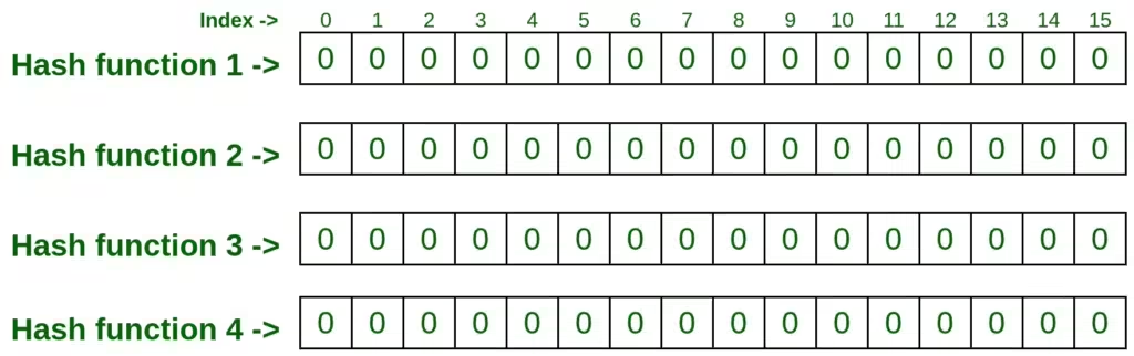
- Hash Functions:
- Multiple hash functions are used to hash each element in the data stream into different “rows” in the sketch. These hash functions are chosen to minimize collisions, which improves the accuracy of the frequency estimates.
- Each element is hashed into d different counters (one per hash function).
- Counters:
- The sketch consists of d rows (where d is the number of hash functions) and w columns (where w is the number of counters per row). Initially, all counters are set to zero.
- Each element’s count is stored by incrementing the corresponding counters for each of the hash functions.
- Frequency Query:
- When querying the frequency of an element, the algorithm computes the minimum count from all the counters that the element was hashed into. This ensures that the query reflects the closest approximation of the actual frequency while avoiding overestimation due to collisions.
- Error Bounds:
- The estimate provided by Count-Min Sketch is an upper bound. The more collisions occur, the higher the estimate might be. The probability of error can be controlled by adjusting the size of the sketch (i.e., w and d).
Key Properties
- Space Efficiency: Count-Min Sketch uses much less space than storing exact frequencies for all elements. The space complexity is O(w * d), where w is the number of columns (related to the desired accuracy) and d is the number of rows (related to the desired confidence).
- Time Efficiency: Updating and querying the sketch are very fast, requiring just O(d) hash computations, making CMS ideal for high-throughput data streams.
- Approximation: The frequency returned is approximate. The sketch guarantees that the estimated frequency is at least the true frequency, and the error is bounded by the number of collisions caused by hashing multiple elements into the same counters.
Applications of Count-Min Sketch
- Network Traffic Monitoring: CMS can be used to approximate the frequency of different IP addresses, packet sizes, or protocol types in high-speed networks, where exact counting might be infeasible.
- Search Engines: In large search indexes, CMS helps track the frequency of query terms, aiding in search term popularity, autocomplete features, and result ranking.
- Recommendation Systems: Online retailers or streaming services can use CMS to approximate the popularity of items or content viewed by users, improving recommendations.
- Database Query Optimization: CMS can track the frequency of database queries to optimize caching strategies or indexing.
- Natural Language Processing: CMS helps track word or phrase frequency in large-scale text processing tasks, making it a good fit for language models or summarization algorithms.
Advantages of Count-Min Sketch
- Memory Efficient: It uses significantly less memory compared to exact counting.
- Speed: Updates and queries are fast, making CMS suitable for real-time applications.
- Scalability: It works well with large-scale data streams.
Disadvantages of Count-Min Sketch
- Overestimation: CMS can overestimate frequencies due to hash collisions.
- Approximate Results: Since it only provides approximate frequencies, it’s unsuitable for applications that require exact counts.
- Hash Function Sensitivity: The performance and accuracy of CMS heavily depend on the choice of hash functions.
Dive into details
Imagine you are managing a data stream of words representing search queries coming into a search engine. Each query might repeat many times, and you want to keep track of how often each word appears. However, storing an exact count for each word is impractical due to memory constraints, especially since the stream is enormous. Instead, we use a Count-Min Sketch to estimate the frequencies.
Let’s say we have the following search queries:
- apple
- banana
- apple
- orange
- banana
- apple
The goal is to approximate the frequency of each word using CMS.
Steps
Step 1: Initialize Count-Min Sketch
A Count-Min Sketch is initialized with two parameters:
- w: The number of columns (width) in the sketch. This defines the number of counters in each row, influencing the accuracy of the estimates.
- d: The number of rows (depth) in the sketch. Each row corresponds to a different hash function, which helps in reducing collisions.
For simplicity, let’s set:
Width (w) = 10 (i.e., 10 counters per row)
Depth (d) = 3 (i.e., 3 rows, each using a different hash function)
Initially, the Count-Min Sketch is a matrix of zeros:
Row 1: [0, 0, 0, 0, 0, 0, 0, 0, 0, 0]
Row 2: [0, 0, 0, 0, 0, 0, 0, 0, 0, 0]
Row 3: [0, 0, 0, 0, 0, 0, 0, 0, 0, 0]
Step 2: Choose Hash Functions
We need three different hash functions (since d=3) to map each word to a counter in each row. These hash functions will map each word to one of the 10 counters in each row. Let’s use simplified hash functions for this example:
Hash Function 1 (Row 1): hash1(“apple”) % 10 = 3
Hash Function 2 (Row 2): hash2(“apple”) % 10 = 7
Hash Function 3 (Row 3): hash3(“apple”) % 10 = 2
For each word, the three hash functions will point to different positions in the three rows, ensuring that the word updates multiple counters.
Step 3: Process the Data Stream
Now, let’s process each word in the stream and update the CMS accordingly.
First word: “apple”: Hashing “apple”:
- Row 1: hash1(“apple”) % 10 = 3 → Increment the 3rd position in Row 1.
- Row 2: hash2(“apple”) % 10 = 7 → Increment the 7th position in Row 2.
- Row 3: hash3(“apple”) % 10 = 2 → Increment the 2nd position in Row 3.
Updated CMS:
Row 1: [0, 0, 0, 1, 0, 0, 0, 0, 0, 0]
Row 2: [0, 0, 0, 0, 0, 0, 0, 1, 0, 0]
Row 3: [0, 0, 1, 0, 0, 0, 0, 0, 0, 0]
Second word: “banana”: Hashing “banana”:
- Row 1: hash1(“banana”) % 10 = 5 → Increment the 5th position in Row 1.
- Row 2: hash2(“banana”) % 10 = 3 → Increment the 3rd position in Row 2.
- Row 3: hash3(“banana”) % 10 = 9 → Increment the 9th position in Row 3.
Updated CMS:
Row 1: [0, 0, 0, 1, 0, 1, 0, 0, 0, 0]
Row 2: [0, 0, 0, 1, 0, 0, 0, 1, 0, 0]
Row 3: [0, 0, 1, 0, 0, 0, 0, 0, 0, 1]
Third word: “apple” (appears again): Hashing “apple”:
- Row 1: Increment the 3rd position in Row 1.
- Row 2: Increment the 7th position in Row 2.
- Row 3: Increment the 2nd position in Row 3.
Updated CMS:
Row 1: [0, 0, 0, 2, 0, 1, 0, 0, 0, 0]
Row 2: [0, 0, 0, 1, 0, 0, 0, 2, 0, 0]
Row 3: [0, 0, 2, 0, 0, 0, 0, 0, 0, 1]
Fourth word: “orange”: Hashing “orange”:
- Row 1:
hash1("orange") % 10 = 4→ Increment the 4th position in Row 1. - Row 2:
hash2("orange") % 10 = 5→ Increment the 5th position in Row 2. - Row 3:
hash3("orange") % 10 = 1→ Increment the 1st position in Row 3.
Updated CMS:
Row 1: [0, 0, 0, 2, 1, 1, 0, 0, 0, 0]
Row 2: [0, 0, 0, 1, 0, 1, 0, 2, 0, 0]
Row 3: [0, 1, 2, 0, 0, 0, 0, 0, 0, 1]
Fifth word: “banana” (appears again): Hashing “banana”:
- Row 1: hash1(“banana”) % 10 = 5 → Increment the 5th position in Row 1.
- Row 2: hash2(“banana”) % 10 = 3 → Increment the 3rd position in Row 2.
- Row 3: hash3(“banana”) % 10 = 9 → Increment the 9th position in Row 3.
Updated CMS after this step:
Row 1: [0, 0, 0, 2, 1, 2, 0, 0, 0, 0]
Row 2: [0, 0, 0, 2, 0, 1, 0, 2, 0, 0]
Row 3: [0, 1, 2, 0, 0, 0, 0, 0, 0, 2]
Sixth word: “apple” (appears again): Hashing “apple”:
- Row 1: hash1(“apple”) % 10 = 3 → Increment the 3rd position in Row 1.
- Row 2: hash2(“apple”) % 10 = 7 → Increment the 7th position in Row 2.
- Row 3: hash3(“apple”) % 10 = 2 → Increment the 2nd position in Row 3.
Final CMS after processing the entire stream:
Row 1: [0, 0, 0, 3, 1, 2, 0, 0, 0, 0]
Row 2: [0, 0, 0, 2, 0, 1, 0, 3, 0, 0]
Row 3: [0, 1, 3, 0, 0, 0, 0, 0, 0, 2]
Step 4: Querying the Count-Min Sketch
Now, let’s query the Count-Min Sketch for the frequency of the words “apple”, “banana”, and “orange”.
Query “apple”:
- Row 1: hash1(“apple”) % 10 = 3 → The count at position 3 in Row 1 is 3.
- Row 2: hash2(“apple”) % 10 = 7 → The count at position 7 in Row 2 is 3.
- Row 3: hash3(“apple”) % 10 = 2 → The count at position 2 in Row 3 is 3.
Estimated frequency of “apple” = min(3, 3, 3) = 3.
Query “banana”:
- Row 1: hash1(“banana”) % 10 = 5 → The count at position 5 in Row 1 is 2.
- Row 2: hash2(“banana”) % 10 = 3 → The count at position 3 in Row 2 is 2.
- Row 3: hash3(“banana”) % 10 = 9 → The count at position 9 in Row 3 is 2.
Estimated frequency of “banana” = min(2, 2, 2) = 2.
Query “orange”:
- Row 1: hash1(“orange”) % 10 = 4 → The count at position 4 in Row 1 is 1.
- Row 2: hash2(“orange”) % 10 = 5 → The count at position 5 in Row 2 is 1.
- Row 3: hash3(“orange”) % 10 = 1 → The count at position 1 in Row 3 is 1.
Estimated frequency of “orange” = min(1, 1, 1) = 1.
Key Points to Note:
- Overestimation: Count-Min Sketch never underestimates the frequency of an element. If there are hash collisions, it will overestimate the count, but it guarantees the estimate is never lower than the true count.
- Space Efficiency: Instead of storing the exact count for each word, which could consume a large amount of memory, CMS only uses a small matrix (in this case, a 3×10 matrix) to approximate the frequencies. This makes it highly space-efficient.
Conclusion
Count-Min Sketch is an effective solution for approximating frequencies in large-scale data streams with constrained memory. By using multiple hash functions and a small set of counters, CMS provides fast and space-efficient frequency estimates. Although there is a trade-off in accuracy (due to possible overestimations from collisions), the error can be controlled by adjusting the size of the sketch.
In scenarios like real-time analytics, network monitoring, or search engine query analysis—where memory is limited and exact counts are not required—Count-Min Sketch offers a powerful, scalable alternative to exact counting.